Support Vector Machines: Start with the Optimal Separating Hyperplane
What is the support vector machine classifier? A practical extension of an ideal classification rule – where the ideal case achieves zero prediction errors, but the extension must compromise via minimal error. The literature calls that ideal classification rule, the “optimal separating hyperplane.” This optimal separating hyperplane must be understood first, before extending to the support vector machine.
In this post, I establish context for the support vector machine’s optimization problem, which I initially find non-intuitive. I essentially share my “margin notes” for The Elements of Statistical Learning Section 4.5.
Visualize an Example Problem
Consider a fundamental example problem. We possess a dataset where each observation has:
- Two features, \((X_1, X_2)\), and
- A class label: +1 or -1.
Our objective is to describe a boundary which “optimally” separates the two classes’ data points. A “decision boundary” arises, as side-of-boundary decides a data point’s class prediction. Your intuition correctly suggests that, an optimal decision boundary keeps far-as-possible from plotted data points. Using new vocabulary, we may call data points’ distance-from-boundary, margin. So a maximum-margin boundary is optimal.
Now invoke a major assumption about the observed data: class labels may be perfectly predicted, by a decision boundary with linear functional form1. This special decision boundary is the “optimal separating hyperplane.”
In the following visual, your eyes properly estimate the horizontal axis as the optimal separating hyperplane.
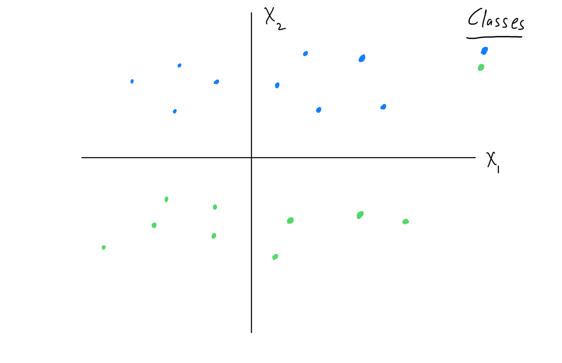
Figure 1: Visualize the optimal separating hyperplane problem.
Derive the Optimal Separating Hyperplane
Let’s derive that special decision boundary which is the optimal separating hyperplane.
Calculate Data Points’ Distance-From-Plane
We must first calculate each data point’s distance-from-plane. This distance calculation follows from a remarkable fact. A data point’s scaled distance-from-plane computes by simply plugging into the plane function. A step-by-step derivation follows.
Point-to-plane distance computes via classic linear algebra procedure:
Identify a length-one vector perpendicular to the plane – a unit normal vector.
Project the point-to-plane vector onto that unit normal vector.
Now, consider the example problem at hand. Remarkably, using problem definitions and some quick operations, we carry out steps (1) and (2).
Start by specifying the plane function, and moving all X inputs to the right-hand side. Writing the multiplication in matrix form generalizes to arbitrarily many X variables.
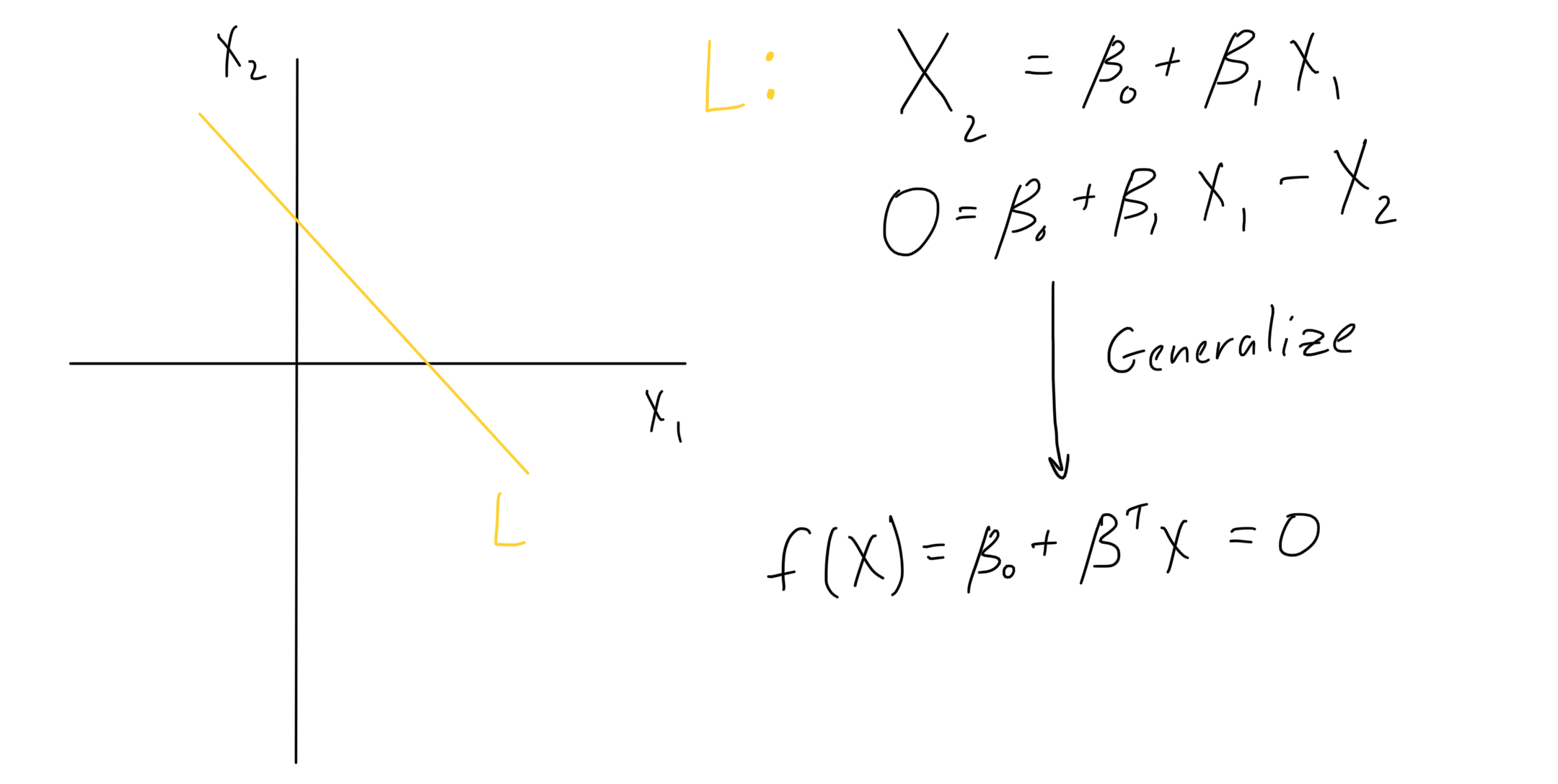
Figure 2: Generalize the plane function, to have arbitrarily many X variables.
To obtain a unit normal vector for the plane, work toward a statement of this object’s definition, by applying operations. Evaluate the function at two points and subtract. From that expression, linear algebra definitions highlight the unit normal vector.
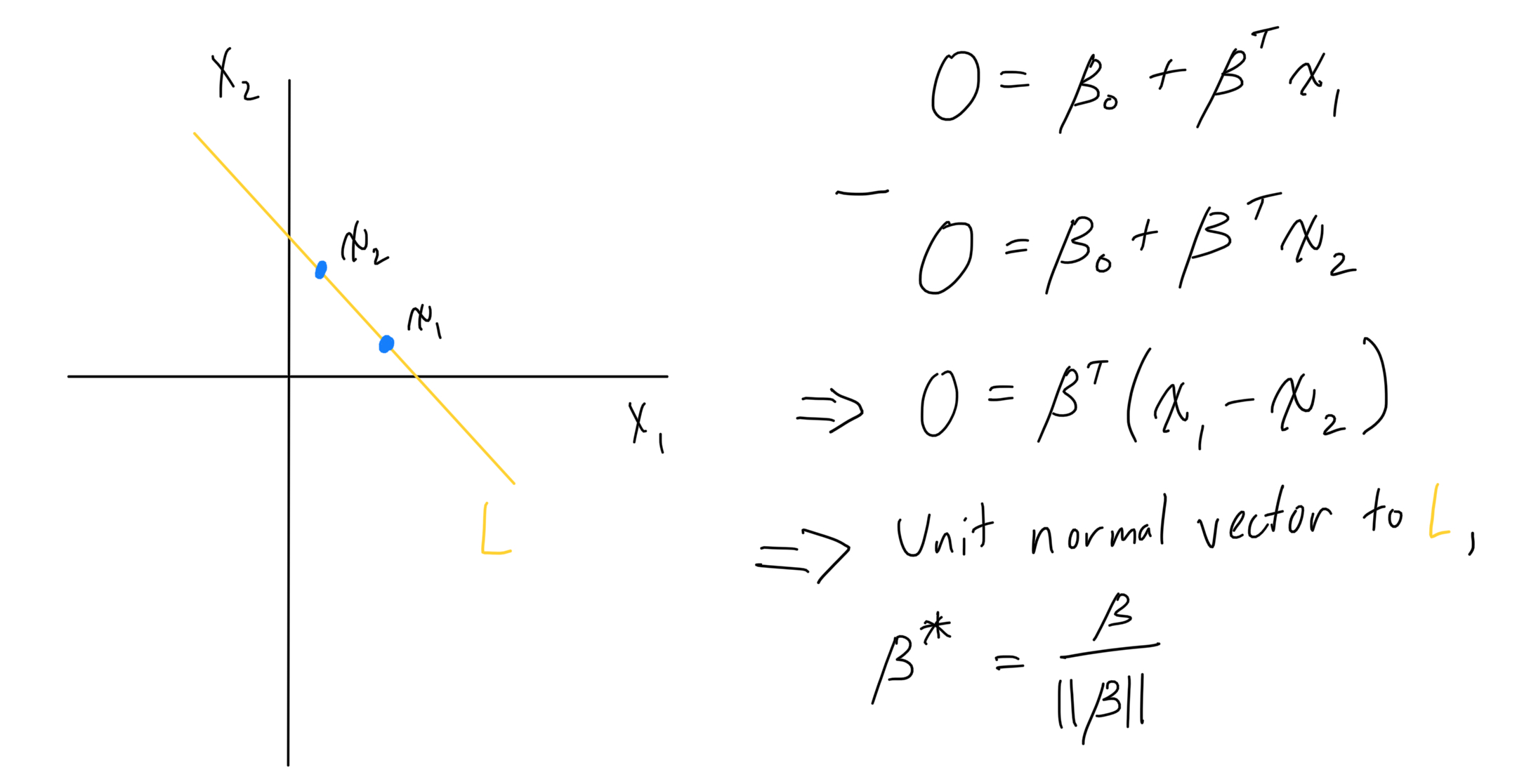
Figure 3: Derive a unit normal vector, using the plane function and linear algebra definitions.
All inputs have been collected to compute point-to-plane distance. Follow the projection formula, and then make substitutions, so it no longer requires an actual point on the plane.
\[ D = (\frac{\beta}{||\beta||})^T (X - X_0) \]
\[ D = (\frac{1}{||\beta||}) (\beta^T X - \beta^T X_0) \]
\[ \text{Recall: } 0 = \beta_0 + \beta^T X \]
\[ \implies D = (\frac{1}{||\beta||}) (\beta^T X + (\beta_0)) \]
\[ \implies D = (\frac{1}{||\beta||}) f(X) \]
(Above statements adapted from Elements of Statistical Learning 4.40).
Using the function which describes the hyperplane decision boundary, we obtain a data point’s scaled distance-from-plane, simply by plugging in predictor values.
Calculate Optimal Separating Hyperplane
The optimal separating hyperplane entails function parameter values – those which enforce data points’ correct classification, and maximize their distance-from-plane (“margin”).
Make an initial statement of the optimization problem, adding one caveat to enforce unique solution:
\[ \text{Definitions: } M = \text{margin}, y_i = \text{class label} \{-1, +1\} \]
\[ \text{Optimize: } \]
\[ \text{max}_{\beta, \beta_0, ||\beta|| = 1} M \]
\[ \text{subject to } y_i(x_i^T \beta + \beta_0) \geq M, i = 1, 2, ..., M \]
(Above statements adapted from Elements of Statistical Learning 4.45).
As \(\beta\) primarily convey the plane’s direction, scaling can produce arbitrarily many solutions. So unit-scaling enforces a unique solution. The “subject to” constraint ensures, for each data point: correct class prediction (negative times negative, or positive times positive), and distance-from-plane (margin) of at least M.
Notice how the constraint set may generalize beyond \(||\beta||=1\). Use our earlier expression for a data point’s distance-from-plane:
\[ \text{Recall: } D = (\frac{1}{||\beta||}) (\beta^T X + (\beta_0)) \]
\[ \text{Re-write constraint: } (\frac{1}{||\beta||}) y_i (x_i^T \beta + \beta_0) \geq M \]
(Above statements adapted from Elements of Statistical Learning 4.46).
Continue simplifying. Continue with the scale-invariance of a solving \(\beta\), and strategically choose a \(\beta\) magnitude:
\[ \text{Declare: } ||\beta|| = 1/M \]
\[ \text{Re-write constraint: } y_i (x_i^T \beta + \beta_0) \geq 1 \]
(Above statements adapted from Elements of Statistical Learning 4.47).
Finally, the original optimization problem may be re-written. With the above declaration, minimum \(\beta\) magnitude achieves maximum margin.
\[ \text{min}_{\beta, \beta_0} \frac{1}{2} ||\beta||^2 \]
\[ \text{subject to } y_i (x_i^T \beta + \beta_0) \geq 1, i = 1, 2, ..., N \]
(Above statements adapted from Elements of Statistical Learning 4.48).
Ultimately, between the decision boundary and surrounding data points, there’s “an empty slab or margin […] of thickness 1/\(||\beta||\)” (ESL). Again in line with intuition, optimal \(\beta\) maximizes that thickness.
The final statement solves using an algorithm. Its implications deliver insight: the solving \(\beta\) are determined by the hyperplane’s closest data point(s). These should matter most, as their classification is relatively least certain.
The final problem statement primes us for the support vector machine extension we’ll see in the next blog post.
Note, a non-linear decision boundary can result from a linear functional form, by properly transforming model inputs.↩︎