Data Drift Detection, from First Principles
TL;DR
How might a data analysis system detect data drift: shifts in data distribution? Depending on context, shifting data distributions may imply new opportunities for fast action, or new risks to be mitigated. In this post, first principles build to an automated drift detection method, tailored for categorical data.
The objective: detect practically significant drift between test and historical population distributions, in light of sample evidence. Even under no population data drift, data samples drift to varying extents. To assess whether one test sample has “critically” drifted, compare to a point of reference: other samples under no population drift (available via simulation). Samples compare automatically because each one reduces to a drift statistic: Kullback-Leibler (KL) Divergence. Then, drift detection alerts when a drift statistic exceeds a critical value, tuned for the application. Reference sample visualizations help with this tuning.
Our “first principles” logic chain parallels hypothesis testing from classical statistics.
For code, see here.
A Data Drift Case Study: Lemons at Carvana
Given two datasets, (1) test and (2) historical – let’s assess data distribution drift. How dissimilar are the test and historical population distributions, in light of the sample evidence? Conclusions depend on the test dataset’s observation count. In smaller data samples, there’s more variability in the drift statistic (KL Divergence, described later). Ultimately we’ll tune an automated method to detect meaningful data drift.
Let’s study real data from Carvana, a car retailer. Around 2012, Carvana posted wholesale auto auction transaction data for a prediction competition. The instruction: “predict if a car purchased at auction is a lemon.” Carvana defines a lemon as a car with “serious issues that prevent it from being sold to customers […] [such as] tampered odometers, mechanical issues the dealer is not able to address, issues with getting the vehicle title from the seller,” etc. In total, Carvana shares about 49,000 test observations and 73,000 historical observations.
Let’s assess drift in car’s Make, specifically.
Manually Assess Distribution Drift, with Entire Data
Let’s first eyeball the extent of drift, using the entire data. This manual assessment helps tune an automated method for live future monitoring.
The probability distribution appears (visually) similar, test versus historical:
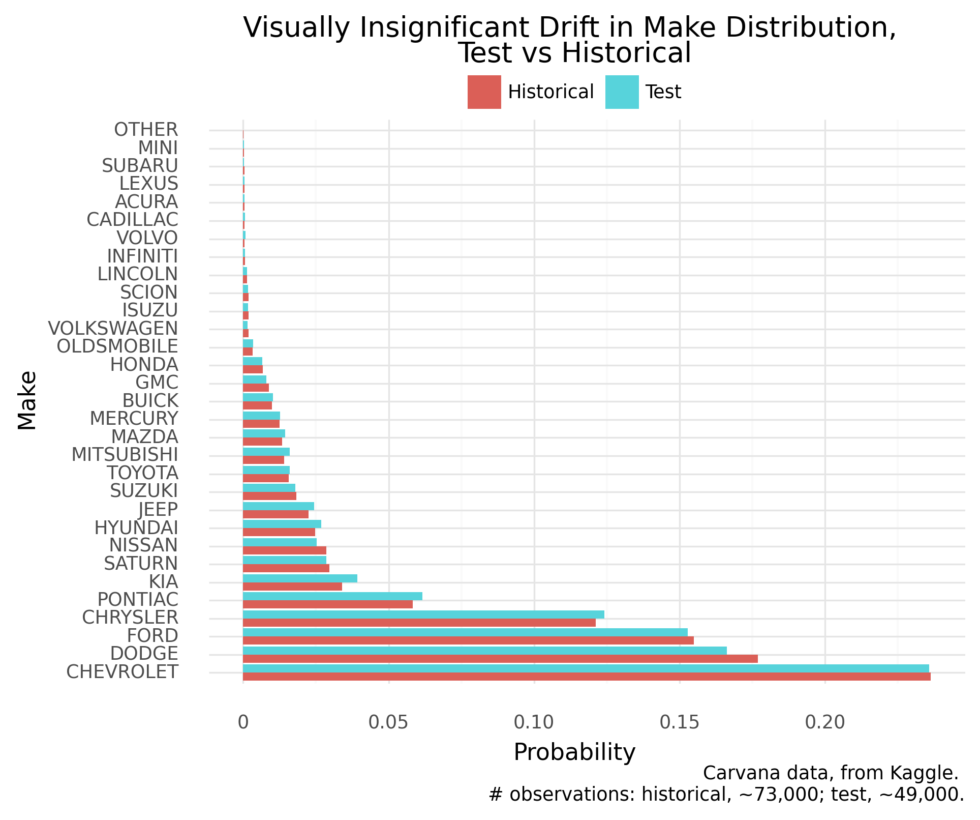
Without deeper domain knowledge to suggest otherwise, let’s adopt the ground truth of no meaningful data drift. The same assessment should arise from a well-tuned automated method.
Statistically, Large Test Data Have Drifted (As Expected)
To assess whether the full test sample has “critically” drifted, we compare to a point of reference: other samples under no population drift (available via simulation). Even under no population data drift, data samples will reflect a range of drift. To start, let’s draw each reference sample to have the same size as the full test sample. Next, each sample reduces to a drift statistic (KL Divergence, described later), allowing easy comparisons.
Turns out, the full test sample drifts more from historical than practically any reference sample under no population drift. Under no population drift, a sample of this size should hardly drift at all:
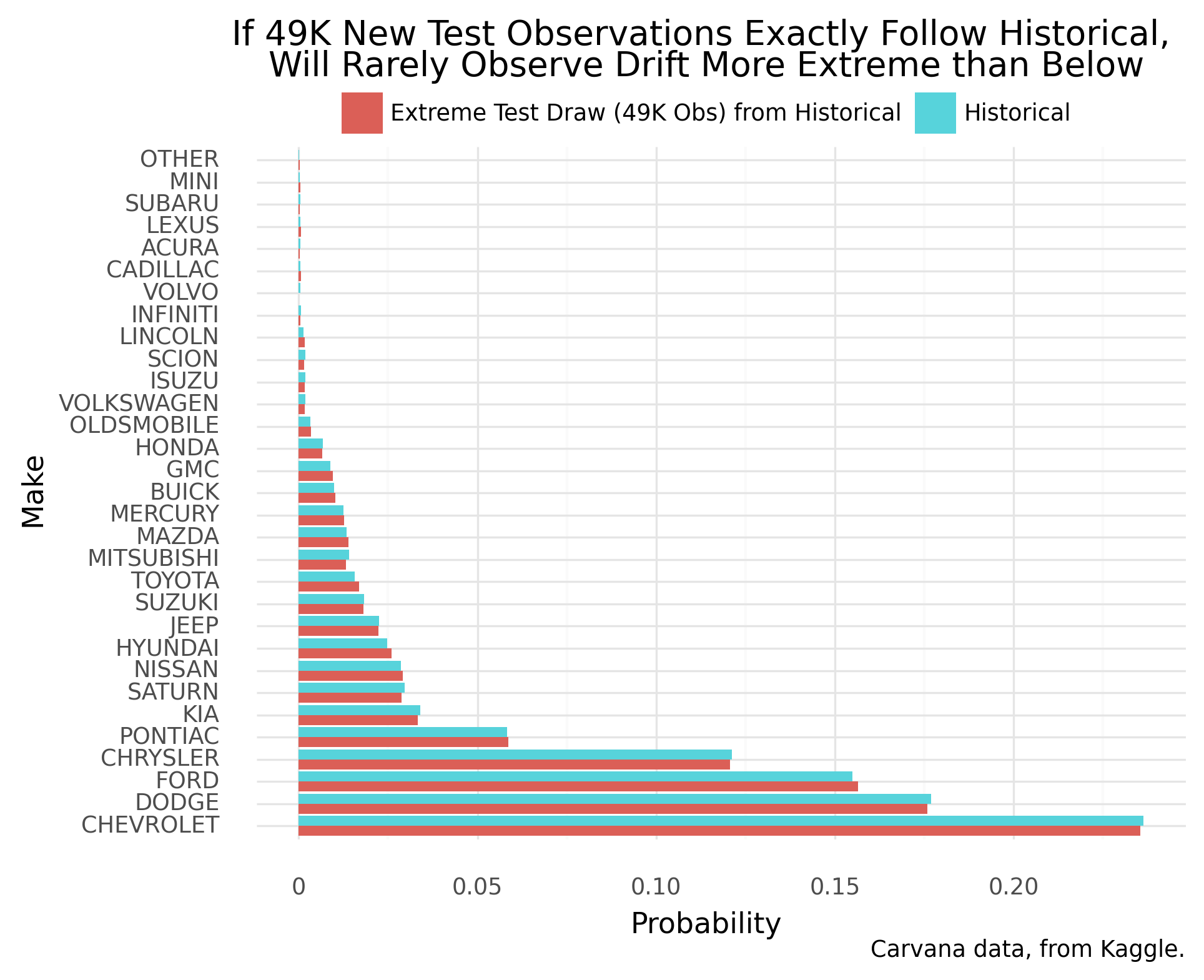
Real, large data might be expected to technically drift–generating processes should be highly dynamic. This theme also appears in other statistical tests of distributions1. So we must tune our method to detect practically significant population drift, above statistically significant drift.
Practical Drift Detection Tunes to Proper Sensitivity
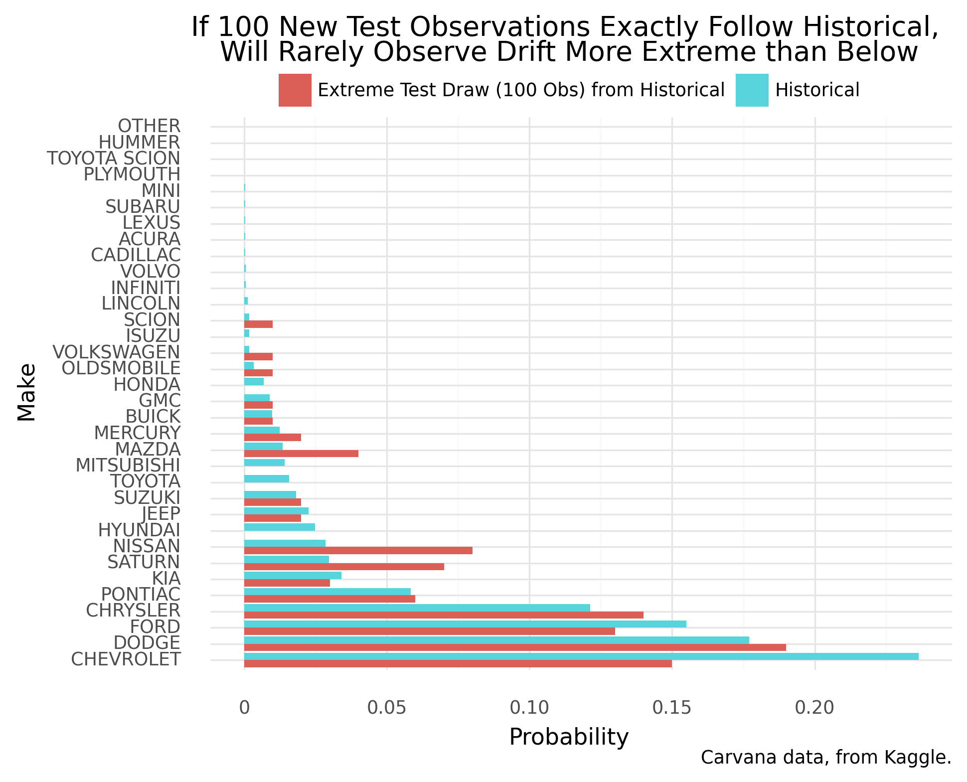
To raise the magnitude of “critical drift” that’s auto-detected, we utilize smaller samples under no population drift. Among smaller data samples, we find larger drift statistics–more sensible critical values. Again a choice of “critical drift” must be visually confirmed for proper sensitivity.
We tune to detect practically significant drift. The following chart shows a proposed tuning for “critical drift”:
In live future monitoring, when a new sample’s drift extremity meets or exceeds above, we’d be automatically alerted.
More method details follow.
KL Divergence Measures Dissimilarity Between Probability Distributions
Suppose we have two probability distributions (a distribution defines the likelihood of generating a data value, over all possible values). To measure the distributions’ dissimilarity, we may:
- compute the difference between their probabilities,
- weight, and
- sum
This procedure formalizes in Kullback-Leibler (KL) Divergence– which intakes probability distributions p and q, and partitions data values by segment k:
\[ KL = \sum_{k=1}^K p_k \log \frac{p_k}{q_k} \]
As a data segment’s probability increasingly differs between the two distributions, the measure rises. And that difference matters more for high-probability segments. Regarding special cases: the measure equals zero when the distributions are identical, or it approaches infinity when a data segment has probability zero under q but nonzero under p.
So KL Divergence is a fast calculation of distributions’ dissimilarity. But how do we make meaning of a KL Divergence value? What’s a large value or a small value?
For Data Drift Test, KL Divergence Meaning is Relative
In data drift testing, KL Divergence’s meaning is relative– relative to its range of values under no population drift. Even under no population drift, data samples’ KL Divergence should vary from zero. And with smaller data samples, KL Divergence should vary more widely. We can estimate the range of sample values under no population drift, by repeated draws of data samples.
KL Divergence’s relative value provides evidence for the question: how much does one probability distribution drift from a baseline distribution? If among no-population drift scenarios, a more extreme KL is rarely seen, then we question the premise of no data drift.
“First Principles” Testing Approach Parallels Classical Hypothesis Testing
With intuition and first principles, we’ve formulated a drift test from KL Divergence. Classical hypothesis testing frames our specific steps:
- Declare a question about population(s) underlying data
- Does one population probability distribution drift from another?
- Propose a baseline (null) hypothesis, to be tested
- Assume no population drift, setting up comparison to other samples under no population drift
- Devise a test statistic, having known range of values under correct null hypothesis (having known sampling distribution)
- Simulate the range of KL Divergence values under no population drift
- Calculate test statistic for observed data sample
- Calculate sample’s KL Divergence
- Measure test statistic relative to its range of values under correct null hypothesis. May compute p-value: probability of a test statistic with equal or greater extremity, assuming correct null hypothesis.
- Measure KL Divergence relative to other samples’ values under no population drift
- Evaluate null hypothesis reasonableness, according to implied likelihood of observed data
- If among no-population drift scenarios, a more extreme KL is rarely seen, then question the premise of no population drift.