Linear Models - A Clearly Linear Business Case Study
Comparing ‘Off-the-Shelf’ Solutions from Classical Statistics and Machine Learning
Key Takeaways
A business case study may be played out using a replicable controlled experiment1.
Consider a hypothetical business case with these characteristics:
- The objective is prediction of a numerical outcome.
- Many indicators are available to try and predict the outcome. However, industry expertise theorizes that only a few particular indicators matter, and those theories are correct.
- The outcome has a truly linear relationship with each relevant predictor (or that predictor raised to a power).
- I analyze example data with “off-the-shelf” linear models from classical statistics and machine learning. The classical statistics model reaches the effective ceiling of prediction performance. The machine learning solution falls well short.
A Business Case Study May Play Out via Controlled Experiment
My earlier post defines a particular type of experiment/simulation. We use the computer to construct a world in which we know the true relationship between predictor(s) and an outcome. With a true relationship defined, random number generation produces data like we would observe in real life: predictor(s) x, and noisily related outcome y. With this level of control – “answer key” in hand – we’re able to understand different models’ relative performance and behavior.
An experiment is interesting when it closely reflects a real-world business case. Then, experimental results help guide real-world decision-making. How can we ensure that an experiment reflects a particular business case? We tailor the details of the experiment’s true relationship. An experiment’s true relationship reflects a highly specific business case. It’s not safe to pull experimental results out of that highly specific context.
A Clearly Linear Business Case Study, via Experiment
Consider the following case study. I prioritize transparency and replicability, so I hope you’ll explore my R code here.
Business Case Details
A manufacturing company executive seeks to predict a production facility’s hourly output. Industry expertise proposes that four factors have predictive power:
- Indoor temperature
- Laborers’ average wage
- Laborers’ average hours of sleep the night before
- Foreman’s average wage
In truth, these are the relevant predictors. Other unrecorded factors impact output in “one-off” ways, adding random noise to the observed outcome.
46 other potential predictors are recorded, but all lack true predictive power. 1,000 data points are available.
The business question – how may output be accurately predicted? Consider two approaches, by discipline:
- Classical statistics, incorporating industry expertise about which predictors matter
- Machine learning, preferring computational power over industry expertise
Step 1: Introduce Training Data
A high-impact data analysis begins with exploration. For example, how do the data look? Plots alone may deliver compelling insights. An interpretable statistical model quantifies visualizable patterns. The alternative is confusion and frustration among model users.
Here, training data plots correctly suggest whether a predictor has a true linear relationship with the outcome.
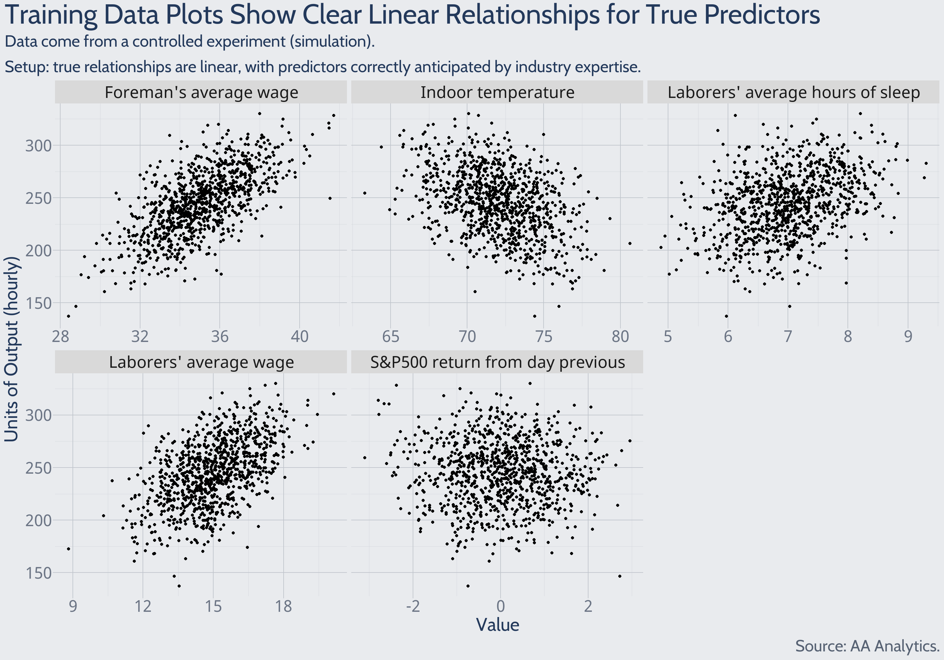
Consider the S&P500 returns plot shown above. It is known from the experimental setup that S&P500 returns are truly unrelated to output. But note the outliers along the plot’s boundaries. Taken with too much weight, these extreme but chance points provoke uncertainty around the claim of zero relationship between S&P500 returns and output. Enforcing the claim of zero relationship amounts to a model simplification. To preview what’s ahead – an overly complex model fails to impose this simplification, and forecast performance suffers.
Step 2: Estimate Models
From the training dataset, I estimate each discipline’s linear model. For apples-to-apples comparison, I want each modeling approach to require a similar level of my time and manual intervention. For the classical statistics model, those requirements are low, and the method requires no customization when pulled off the discipline’s “shelf.” The machine learning model pulled from the “shelf” requires some customization choices – I use experts’ published code defaults. Said another way, I adopt generally “off-the-shelf” estimation approaches. For more details:
Begin with the big picture.
When estimating the classical statistics linear model, incorporate industry expertise about which predictors matter. This means that 46 of the potential predictors are properly left out of the model.
When estimating the machine learning linear model, prefer computational power over industry expertise. This means that the algorithm decides which of the 50 predictors are important, and includes those in the model.
Technical details are important for deeper future studies.
Step 3: Evaluate Estimated Models
One metric to summarize prediction performance
Intuitively, we want a model whose prediction errors have low (1) dispersion and (2) average magnitude. How might we summarize these prediction error characteristics? Consider the mean squared error (MSE) metric. This metric increases when there’s an increase in prediction errors’ (1) dispersion or (2) average magnitude. The calculation mirrors the name:
- Square each individual error
- Take the average
To be explicit - when we use MSE to compare different models, the lower value wins.
Predictions of Training Data
Using the calculated models, and predictor values from the training data, we may predict outcomes from the training data. These predictions benefit from hindsight – either model studied the training data to estimate predictor-outcome relationships. These are “backward-looking” predictions, essentially aiming to explain past outcomes.
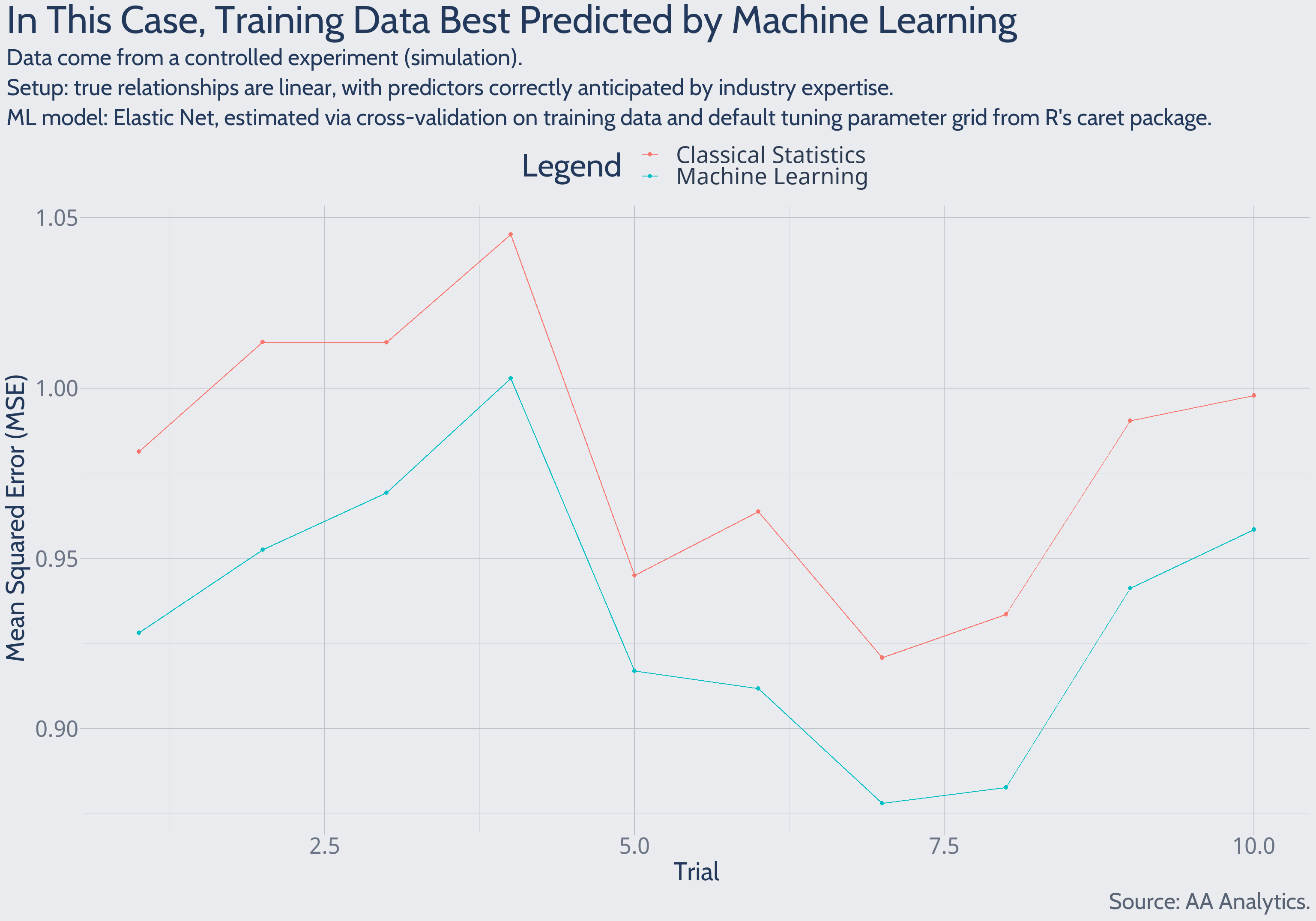
Zooming in on early experimental trials: the machine learning solution explains past data more accurately than the classical statistics solution does. This pattern holds in each of 1,000 total experimental trials.
Predictions of Test Data
Using the calculated models, and predictor values from new test data, we may forecast new outcomes. These test data are encountered strictly after model estimation, so predictions constitute genuine forecasts.
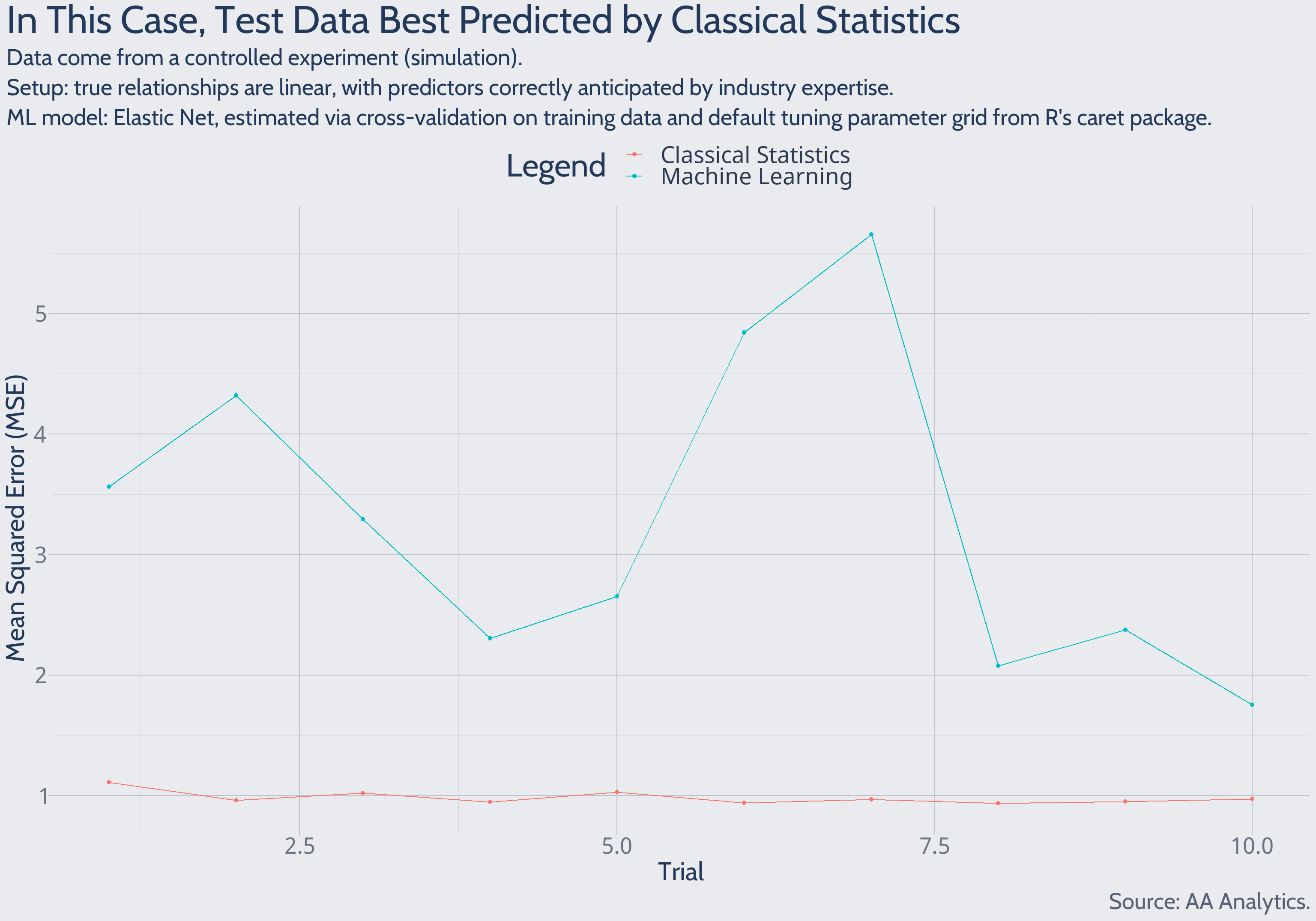
Zooming in on early experimental trials: the classical statistics solution forecasts future data more accurately than the machine learning solution does. This pattern holds in each of 1,000 total experimental trials.
Discussion of Results
Test Data Gauge Whether a Model Learned Real Patterns
By backward-looking prediction performance alone, the machine learning solution edges out classical statistics. However, the classical statistics solution dominates when forecasting outcomes yet to be observed. What explains this phenomenon? A complex model may easily mistake random chance for real predictor-outcome relationships. For a visual example of how randomness may mislead, see the S&P500 returns plot/text above, in “Step 1: Introduce Training Data.” Real patterns are those borne out in new data – so test data properly gauge whether a model has learned real patterns.
Classical Statistics Reaches Prediction Performance Ceiling
The classical statistics model reaches the effective ceiling of prediction performance. Evidence for this claim extends much deeper than the performance relative to machine learning. Observe the earlier “Predictions of Test Data” plot, showing experimental trials’ mean squared error (MSE). The value hovers around 1. Why? MSE estimates the level of random noise in the outcome. Here, because we defined the true level of random noise in the experimental setup, we know this estimate is highly accurate. So it appears the classical statistics model properly distinguishes the outcome’s two sources of variation:
- Variation in the predictors that matter
- Surprise one-off factors
A model’s predictive accuracy may improve only until the relationships in (1) are estimated without error. For our case study’s applied purpose, the classical statistics linear model has reached that point. With no room left for meaningful improvement, any competing model seeks simply to match the classical statistics performance.
“Off-the-Shelf” Machine Learning Approach Needs Customized
Why is this “off-the-shelf” machine learning model better at explaining the past but far worse at forecasting the future? Additional action must be taken to restrict machine learning from mistaking random chance for signal about the future. A more custom approach should help move toward the classical statistics model’s performance ceiling.
Additional explanation of the machine learning result is more technical. To decrease risk of mistaking random chance for signal about the future, model estimation should become a more involved process, with the introduction of validation data. Suppose this business case included more data points – 10,000, for example. We could dedicate two-thirds of these to model training and form initial impressions of model accuracy. Then, the data’s remaining one-third – validation data – better gauges model accuracy. Why? The model did not study the validation data to learn predictor-outcome relationships, so these predictions are more like true forecasts. Iterative model re-formulation, following custom paths, may continue until model accuracy satisfies in both training and validation data. In sum, the analyst better understands model performance beyond the training data, but before encountering formal test data.
It’s common practice to estimate machine learning models without validation data, especially when few data points are available (Zou 2004) (310). Ideally, estimation does include validation data (Hastie 2017) (Section 7.2, 222). This experiment seems to suggest elevated risk when estimating machine learning models without validation data.
References
Hastie, Trevor; Robert Tibshirani; Jerome Friedman. 2017. The Elements of Statistical Learning.
Zou, Hui; Trevor Hastie. 2004. “Regularization and Variable Selection via the Elastic Net.” https://web.stanford.edu/~hastie/Papers/B67.2%20(2005)%20301-320%20Zou%20&%20Hastie.pdf.