Linear Models - A Primer

Classical Statistics and Machine Learning Varieties

Last updated on Oct 16, 2021 5 min read linear regression, estimation, statistics, machine learning, simulation

Key Takeaways

A linear model – a “line of best fit” – estimates the true relationship between predictors and an outcome.
Linear models come in classical statistics or machine learning varieties.
To learn about linear models’ relative performance/behavior, we use controlled experiments, powered by computer simulation.

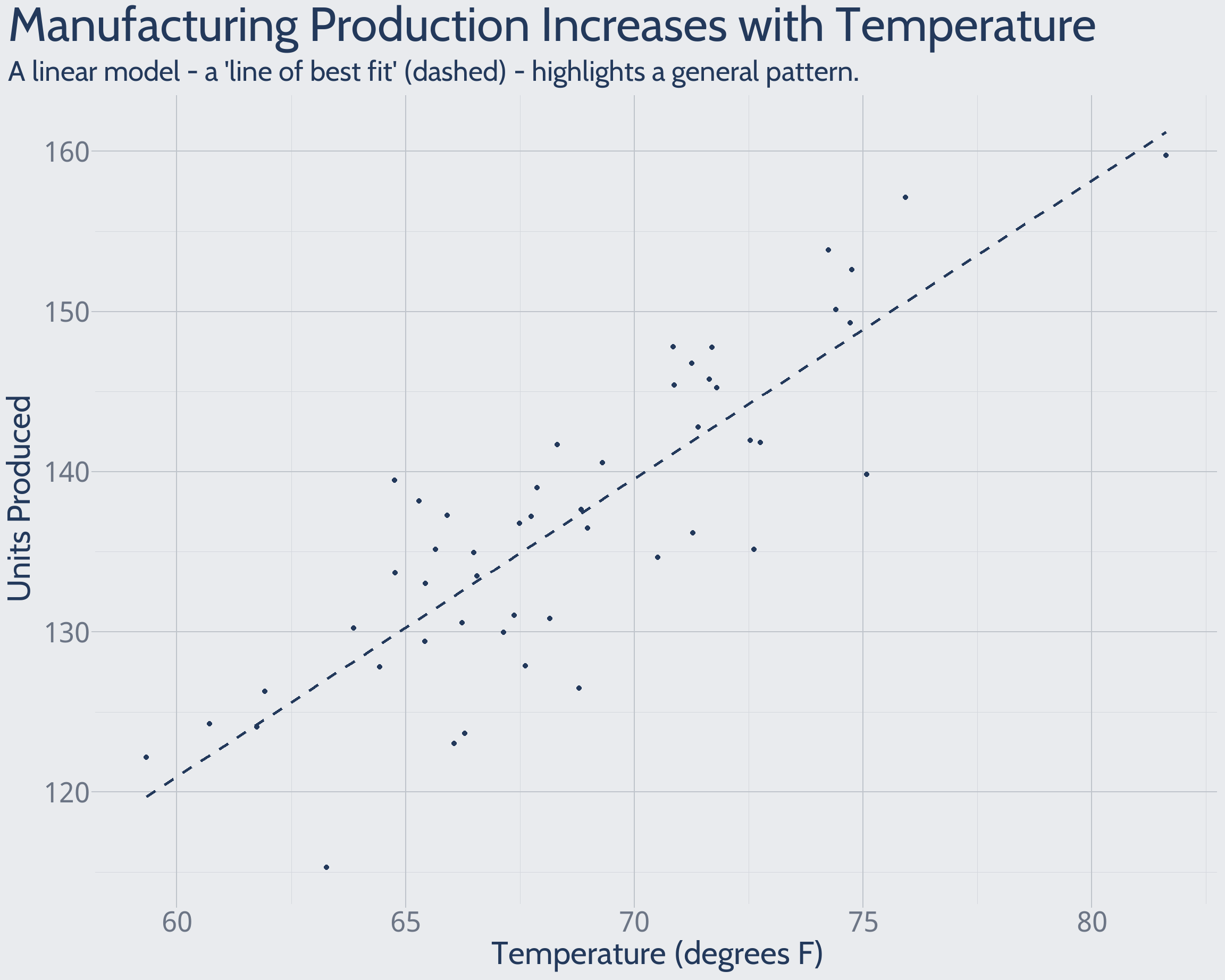
A Linear Model is a “Line of Best Fit”

A linear model is a line of best fit, relating a predictor (x) and an outcome (y). Your eyes likely anticipate this line before it’s drawn. Formally, a linear model is a rule by which x predicts y, minimizing error. The method extends naturally to analyze multiple predictors of an outcome.

Some hypothetical data illustrate the idea:

A Linear Model Estimates an Unknown True Relationship

Fundamentally, a linear model estimates the true relationship between predictor(s) (x) and an outcome (y). In reality, we lack absolute certainty about the true relationship: other relevant factors vary and add random noise to the observed outcome. We use available data to – in the lingo – make inferences about the true relationship.

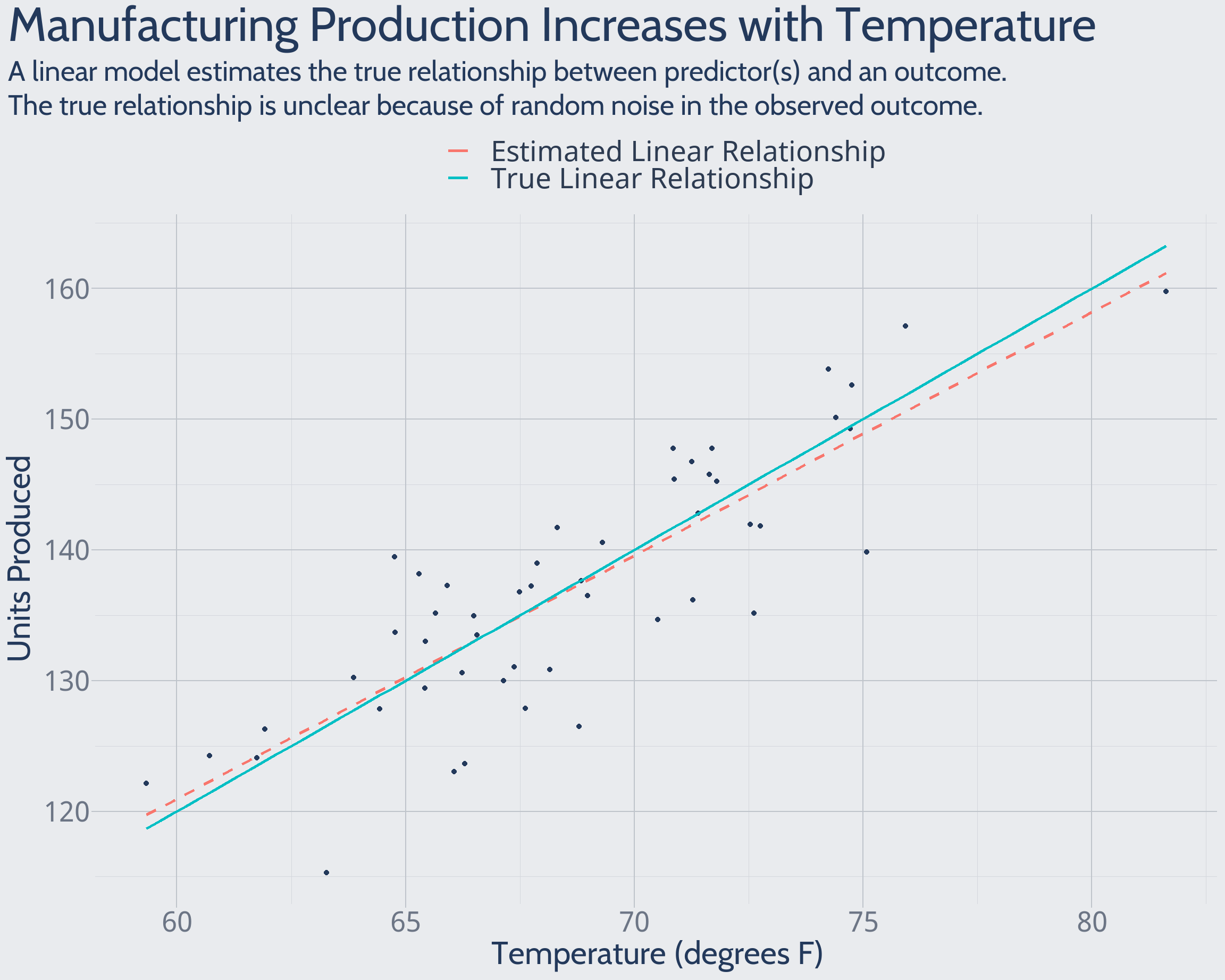
Our critical thinking deepens when we distinguish between (a) the true x-y relationship and (b) the statistically estimated x-y relationship. The distinction provokes a crucial question: how well does a statistical estimate approximate the true relationship?

Thinking in this way also provides the basis for controlled experiments in future work. Essentially, we use the computer to construct a world in which we know the true relationship between predictor(s) and an outcome. With this “answer key” in hand, we’re able to clearly understand different models’ relative performance and behavior.

Linear Models Come in Classical Statistics or Machine Learning Varieties

Both classical statistics and machine learning disciplines propose techniques for linear model estimation. They possess key similarities as well as differences.

Table 1: Linear Model Characteristics by Discipline
Characteristic	Classical Statistics Variety	Machine Learning Variety
Essence	A rule by which x predicts y, minimizing error	A rule by which x predicts y, minimizing error plus a measure of model flexibility
Typical goal	Test whether a relationship between x and y truly exists	Automated search for best potential predictors of y
Source: AA Analytics.

Machine learning’s increased flexibility creates exciting automation opportunities. One sacrifice, though, is classical statistics’ well-defined testing of whether an x-y relationship differs from zero in a “statistically significant” way.

The two disciplines’ linear model techniques also have distinct numerical properties.

Table 2: Linear Model Numerical Properties by Discipline
Numerical Property	Classical Statistics Variety	Machine Learning Variety
Calculation formula	Well-defined (one formula to compute any best-fit line)	Flexible (no one formula minimizes prediction errors plus model flexibility)
Estimation behavior	Model stability improves with more data Under key assumptions, quantify closeness of estimated and true lines	Model stability improves with more data
Source: AA Analytics.

Classical statistics’ single linear model formula implies generally high-speed calculations. Machine learning calculations are relatively slower. In terms of estimation behavior: (1) regardless of discipline, we place more trust in a linear model estimated from 1,000 data points, versus 10. (2) As seen previously, classical statistics is characterized by well-defined testing for “statistically significant” x-y relationships. On the other hand, machine learning prioritizes an intense search for potentially predictive patterns.

Controlled Experiments Enable Studies of Linear Model Behaviors

How can we learn more about linear model behaviors? By experiments¹. We use the computer to construct a world in which we know the true relationship between predictor(s) and an outcome. With this “answer key” in hand, we’re able to clearly understand different models’ relative performance and behavior.

The general structure of an experiment follows.

One trial in an experiment is like one real data analysis project

One trial is the building block of a larger experiment. One trial is essentially one real-world data analysis project.

Table 3: One Trial of a Controlled Numerical Experiment Parallels a Real Data Analysis Project
Step	Real Project	Experimental Trial
1	Collect some data, which follows a true relationship we don’t know.	Generate some data, which follows a true relationship we do know.
2	Estimate linear model(s) from ‘training data’ in (1)	Estimate linear model(s) from ‘training data’ in (1)
3	Evaluate estimated models	Evaluate estimated models
Source: AA Analytics.

The key difference occurs in Step 1. In the real world, data to be modeled (“training data”) already exist, so they’re collected. In an experiment, the true x-y relationship must be written in the computer program. With this true relationship defined, random number generation produces data like we would observe in real life: predictor(s) x, and noisily related outcome y.

Step 3 model evaluation partly entails this question: how well does x predict y, among (a) the training data, and (b) new, never-before-seen “test data”?

One trial involves two distinct datasets: training and test

It is worth highlighting the two distinct datasets involved in an experimental trial.

Table 4: Two Distinct Datasets: Training and Test
Characteristic	Training Data	Test Data
Used to estimate the model?	Yes	No
Nature of associated model predictions	Explaining the past	Forecasting the future
Source: AA Analytics.

Critically, training data are used to estimate² a model. Therefore, any predictions made on these data have the benefit of hindsight. Test data, on the other hand, are never used to estimate the model. So predictions on these data are true forecasts.

A figurative wall separates the training and test datasets.

Figure 1: Inspired by (Hastie 2017).

Repeating many trials averages out random chance results

An experiment repeats many trials, to average out results due to random chance. Then, robust takeaways about model behavior become clearer. To be explicit, what components vary trial-to-trial?

In the training data, noise that muddies y
In the test data, both x and y

References

Hastie, Trevor; Robert Tibshirani; Jerome Friedman. 2017. The Elements of Statistical Learning.

Controlled experiments/simulations are called Monte Carlo experiments, in the lingo.↩︎
“Estimating” a model may also be called “training” or “teaching” a model.↩︎

linear regression estimation statistics machine learning simulation